Python机器学习之SVM支持向量机
SVM支持向量机是建立于统计学习理论上的一种分类算法,适合与处理具备高维特征的数据集。
SVM算法的数学原理相对比较复杂,好在由于SVM算法的研究与应用如此火爆,CSDN博客里也有大量的好文章对此进行分析,下面给出几个本人认为讲解的相当不错的:
支持向量机通俗导论(理解SVM的3层境界)
JULY大牛讲的是如此详细,由浅入深层层推进,以至于关于SVM的原理,我一个字都不想写了。。强烈推荐。
还有一个比较通俗的简单版本的:手把手教你实现SVM算法
SVN原理比较复杂,但是思想很简单,一句话概括,就是通过某种核函数,将数据在高维空间里寻找一个最优超平面,能够将两类数据分开。
针对不同数据集,不同的核函数的分类效果可能完全不一样。可选的核函数有这么几种:
线性函数:形如K(x,y)=x*y这样的线性函数;
多项式函数:形如K(x,y)=[(x·y)+1]^d这样的多项式函数;
径向基函数:形如K(x,y)=exp(-|x-y|^2/d^2)这样的指数函数;
Sigmoid函数:就是上一篇文章中讲到的Sigmoid函数。
我们就利用之前的几个数据集,直接给出Python代码,看看运行效果:
测试1:身高体重数据
# -*- coding: utf-8 -*-
import numpy as np
import scipy as sp
from sklearn import svm
from sklearn.cross_validation import train_test_split
import matplotlib.pyplot as plt

data  = []
labels = []
with open("data\\1.txt") as ifile:
    for line in ifile:
      tokens = line.strip().split(' ')
      data.append([float(tk) for tk in tokens[:-1]])
      labels.append(tokens[-1])
x = np.array(data)
labels = np.array(labels)
y = np.zeros(labels.shape)
y[labels=='fat']=1
x_train, x_test, y_train, y_test = train_test_split(x, y, test_size = 0.0)

h = .02
# create a mesh to plot in
x_min, x_max = x_train[:, 0].min() - 0.1, x_train[:, 0].max() + 0.1
y_min, y_max = x_train[:, 1].min() - 1, x_train[:, 1].max() + 1
xx, yy = np.meshgrid(np.arange(x_min, x_max, h),
           np.arange(y_min, y_max, h))

''''' SVM '''
# title for the plots
titles = ['LinearSVC (linear kernel)',
     'SVC with polynomial (degree 3) kernel',
     'SVC with RBF kernel',
     'SVC with Sigmoid kernel']
clf_linear = svm.SVC(kernel='linear').fit(x, y)
#clf_linear = svm.LinearSVC().fit(x, y)
clf_poly  = svm.SVC(kernel='poly', degree=3).fit(x, y)
clf_rbf   = svm.SVC().fit(x, y)
clf_sigmoid = svm.SVC(kernel='sigmoid').fit(x, y)

for i, clf in enumerate((clf_linear, clf_poly, clf_rbf, clf_sigmoid)):
  answer = clf.predict(np.c_[xx.ravel(), yy.ravel()])
  print(clf)
  print(np.mean( answer == y_train))
  print(answer)
  print(y_train)

  plt.subplot(2, 2, i + 1)
  plt.subplots_adjust(wspace=0.4, hspace=0.4)

  # Put the result into a color plot
  z = answer.reshape(xx.shape)
  plt.contourf(xx, yy, z, cmap=plt.cm.Paired, alpha=0.8)

  # Plot also the training points
  plt.scatter(x_train[:, 0], x_train[:, 1], c=y_train, cmap=plt.cm.Paired)
  plt.xlabel(u'身高')
  plt.ylabel(u'体重')
  plt.xlim(xx.min(), xx.max())
  plt.ylim(yy.min(), yy.max())
  plt.xticks(())
  plt.yticks(())
  plt.title(titles[i])

plt.show()
运行结果如下:
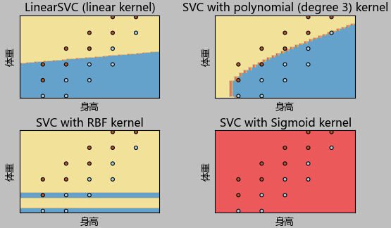
可以看到,针对这个数据集,使用3次多项式核函数的SVM,得到的效果最好。
测试2:影评态度
下面看看SVM在康奈尔影评数据集上的表现:(代码略)
SVC(C=1.0, cache_size=200, class_weight=None, coef0=0.0, degree=3, gamma=0.0, kernel='linear', max_iter=-1, probability=False, random_state=None,
shrinking=True, tol=0.001, verbose=False)
0.814285714286
SVC(C=1.0, cache_size=200, class_weight=None, coef0=0.0, degree=3, gamma=0.0, kernel='poly', max_iter=-1, probability=False, random_state=None, shrinking=True, tol=0.001, verbose=False)
0.492857142857
SVC(C=1.0, cache_size=200, class_weight=None, coef0=0.0, degree=3, gamma=0.0, kernel='rbf', max_iter=-1, probability=False, random_state=None, shrinking=True, tol=0.001, verbose=False)
0.492857142857
SVC(C=1.0, cache_size=200, class_weight=None, coef0=0.0, degree=3, gamma=0.0, kernel='sigmoid', max_iter=-1, probability=False, random_state=None,
shrinking=True, tol=0.001, verbose=False)
0.492857142857
可见在该数据集上,线性分类器效果最好。
测试3:圆形边界
最后我们测试一个数据分类边界为圆形的情况:圆形内为一类,原型外为一类。看这类非线性的数据SVM表现如何:
测试数据生成代码如下所示:
''''' 数据生成 '''
h = 0.1
x_min, x_max = -1, 1
y_min, y_max = -1, 1
xx, yy = np.meshgrid(np.arange(x_min, x_max, h),
           np.arange(y_min, y_max, h))
n = xx.shape[0]*xx.shape[1]
x = np.array([xx.T.reshape(n).T, xx.reshape(n)]).T
y = (x[:,0]*x[:,0] + x[:,1]*x[:,1] < 0.8)
y.reshape(xx.shape)

x_train, x_test, y_train, y_test\
  = train_test_split(x, y, test_size = 0.2)
测试结果如下:
SVC(C=1.0, cache_size=200, class_weight=None, coef0=0.0, degree=3, gamma=0.0, kernel='linear', max_iter=-1, probability=False, random_state=None,
shrinking=True, tol=0.001, verbose=False)
0.65
SVC(C=1.0, cache_size=200, class_weight=None, coef0=0.0, degree=3, gamma=0.0, kernel='poly', max_iter=-1, probability=False, random_state=None,
shrinking=True, tol=0.001, verbose=False)
0.675
SVC(C=1.0, cache_size=200, class_weight=None, coef0=0.0, degree=3, gamma=0.0, kernel='rbf', max_iter=-1, probability=False, random_state=None,
shrinking=True, tol=0.001, verbose=False)
0.9625
SVC(C=1.0, cache_size=200, class_weight=None, coef0=0.0, degree=3, gamma=0.0, kernel='sigmoid', max_iter=-1, probability=False, random_state=None,
shrinking=True, tol=0.001, verbose=False)
0.65
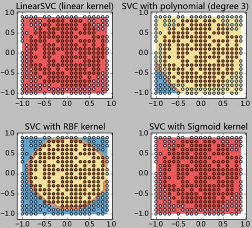
可以看到,对于这种边界,径向基函数的SVM得到了近似完美的分类结果。而其他的分类器显然束手无策。
以上就是本文的全部内容,希望对大家的学习有所帮助,也希望大家多多支持【听图阁-专注于Python设计】。