Tensorflow使用支持向量机拟合线性回归
支持向量机可以用来拟合线性回归。
相同的最大间隔(maximum margin)的概念应用到线性回归拟合。代替最大化分割两类目标是,最大化分割包含大部分的数据点(x,y)。我们将用相同的iris数据集,展示用刚才的概念来进行花萼长度与花瓣宽度之间的线性拟合。
相关的损失函数类似于max(0,|yi-(Axi+b)|-ε)。ε这里,是间隔宽度的一半,这意味着如果一个数据点在该区域,则损失等于0。
# SVM Regression
#----------------------------------
#
# This function shows how to use TensorFlow to
# solve support vector regression. We are going
# to find the line that has the maximum margin
# which INCLUDES as many points as possible
#
# We will use the iris data, specifically:
# y = Sepal Length
# x = Pedal Width

import matplotlib.pyplot as plt
import numpy as np
import tensorflow as tf
from sklearn import datasets
from tensorflow.python.framework import ops
ops.reset_default_graph()

# Create graph
sess = tf.Session()

# Load the data
# iris.data = [(Sepal Length, Sepal Width, Petal Length, Petal Width)]
iris = datasets.load_iris()
x_vals = np.array([x[3] for x in iris.data])
y_vals = np.array([y[0] for y in iris.data])

# Split data into train/test sets
train_indices = np.random.choice(len(x_vals), round(len(x_vals)*0.8), replace=False)
test_indices = np.array(list(set(range(len(x_vals))) - set(train_indices)))
x_vals_train = x_vals[train_indices]
x_vals_test = x_vals[test_indices]
y_vals_train = y_vals[train_indices]
y_vals_test = y_vals[test_indices]

# Declare batch size
batch_size = 50

# Initialize placeholders
x_data = tf.placeholder(shape=[None, 1], dtype=tf.float32)
y_target = tf.placeholder(shape=[None, 1], dtype=tf.float32)

# Create variables for linear regression
A = tf.Variable(tf.random_normal(shape=[1,1]))
b = tf.Variable(tf.random_normal(shape=[1,1]))

# Declare model operations
model_output = tf.add(tf.matmul(x_data, A), b)

# Declare loss function
# = max(0, abs(target - predicted) + epsilon)
# 1/2 margin width parameter = epsilon
epsilon = tf.constant([0.5])
# Margin term in loss
loss = tf.reduce_mean(tf.maximum(0., tf.subtract(tf.abs(tf.subtract(model_output, y_target)), epsilon)))

# Declare optimizer
my_opt = tf.train.GradientDescentOptimizer(0.075)
train_step = my_opt.minimize(loss)

# Initialize variables
init = tf.global_variables_initializer()
sess.run(init)

# Training loop
train_loss = []
test_loss = []
for i in range(200):
  rand_index = np.random.choice(len(x_vals_train), size=batch_size)
  rand_x = np.transpose([x_vals_train[rand_index]])
  rand_y = np.transpose([y_vals_train[rand_index]])
  sess.run(train_step, feed_dict={x_data: rand_x, y_target: rand_y})

  temp_train_loss = sess.run(loss, feed_dict={x_data: np.transpose([x_vals_train]), y_target: np.transpose([y_vals_train])})
  train_loss.append(temp_train_loss)

  temp_test_loss = sess.run(loss, feed_dict={x_data: np.transpose([x_vals_test]), y_target: np.transpose([y_vals_test])})
  test_loss.append(temp_test_loss)
  if (i+1)%50==0:
    print('-----------')
    print('Generation: ' + str(i+1))
    print('A = ' + str(sess.run(A)) + ' b = ' + str(sess.run(b)))
    print('Train Loss = ' + str(temp_train_loss))
    print('Test Loss = ' + str(temp_test_loss))

# Extract Coefficients
[[slope]] = sess.run(A)
[[y_intercept]] = sess.run(b)
[width] = sess.run(epsilon)

# Get best fit line
best_fit = []
best_fit_upper = []
best_fit_lower = []
for i in x_vals:
 best_fit.append(slope*i+y_intercept)
 best_fit_upper.append(slope*i+y_intercept+width)
 best_fit_lower.append(slope*i+y_intercept-width)

# Plot fit with data
plt.plot(x_vals, y_vals, 'o', label='Data Points')
plt.plot(x_vals, best_fit, 'r-', label='SVM Regression Line', linewidth=3)
plt.plot(x_vals, best_fit_upper, 'r--', linewidth=2)
plt.plot(x_vals, best_fit_lower, 'r--', linewidth=2)
plt.ylim([0, 10])
plt.legend(loc='lower right')
plt.title('Sepal Length vs Pedal Width')
plt.xlabel('Pedal Width')
plt.ylabel('Sepal Length')
plt.show()

# Plot loss over time
plt.plot(train_loss, 'k-', label='Train Set Loss')
plt.plot(test_loss, 'r--', label='Test Set Loss')
plt.title('L2 Loss per Generation')
plt.xlabel('Generation')
plt.ylabel('L2 Loss')
plt.legend(loc='upper right')
plt.show()
输出结果:
-----------
Generation: 50
A = [[ 2.91328382]] b = [[ 1.18453276]]
Train Loss = 1.17104
Test Loss = 1.1143
-----------
Generation: 100
A = [[ 2.42788291]] b = [[ 2.3755331]]
Train Loss = 0.703519
Test Loss = 0.715295
-----------
Generation: 150
A = [[ 1.84078252]] b = [[ 3.40453291]]
Train Loss = 0.338596
Test Loss = 0.365562
-----------
Generation: 200
A = [[ 1.35343242]] b = [[ 4.14853334]]
Train Loss = 0.125198
Test Loss = 0.16121
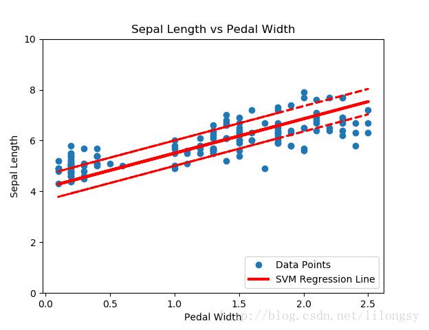
基于iris数据集(花萼长度和花瓣宽度)的支持向量机回归,间隔宽度为0.5
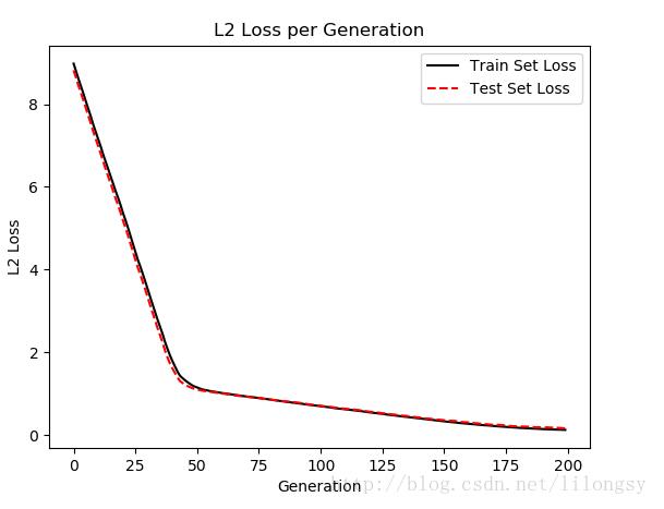
每次迭代的支持向量机回归的损失值(训练集和测试集)
直观地讲,我们认为SVM回归算法试图把更多的数据点拟合到直线两边2ε宽度的间隔内。这时拟合的直线对于ε参数更有意义。如果选择太小的ε值,SVM回归算法在间隔宽度内不能拟合更多的数据点;如果选择太大的ε值,将有许多条直线能够在间隔宽度内拟合所有的数据点。作者更倾向于选取更小的ε值,因为在间隔宽度附近的数据点比远处的数据点贡献更少的损失。
以上就是本文的全部内容,希望对大家的学习有所帮助,也希望大家多多支持【听图阁-专注于Python设计】。